Introduction Software, such as specific R packages, evolve over time, which may prevent older analysis code from working as expected. For example, default values for arguments in a function can change. Therefore, for computational reproducibility, knowing which specific R and package versions were used to run the analysis is crucial. One popular solution in R… Read More
Expanding the Lifespan of Software for Demographic Analysis with Containers: An Application of Spatial Sampling
![Figure 1. Reproducibility struggles. Left: Three laptops showing different software configurations, symbolizing challenges in reproducing results. Right: A single laptop displaying multiple virtual containers with distinct software setups, highlighting improved reproducibility.](https://population-dynamics-lab.csde.washington.edu/wp-content/uploads/2024/04/fig_01_error_v_container-1200x600.png)
Unlocking Population Estimation Using Readily Available Data: Applying the Simplified Censal Ratio Method
![Figure 2: Figure 2 shows a graph depicting the correlation between the Censal Ratio Population estimate of 2019 (based on 2010 data) and the actual US Census Bureau’s 2019 population estimate of 2019. The x-axis shows a range of the 2019 censal ratio population estimate, ranging from 0 to 800,000. The y-axis shows a range of the 2019 population estimate and also ranges from 0 to 800,000. The graph demonstrates how the Censal Ratio Method produces a more closely accurate set of estimations than the symptomatic indicator alone.](https://population-dynamics-lab.csde.washington.edu/wp-content/uploads/2024/04/censal_ratio_to_pop_plot-1200x1047.png)
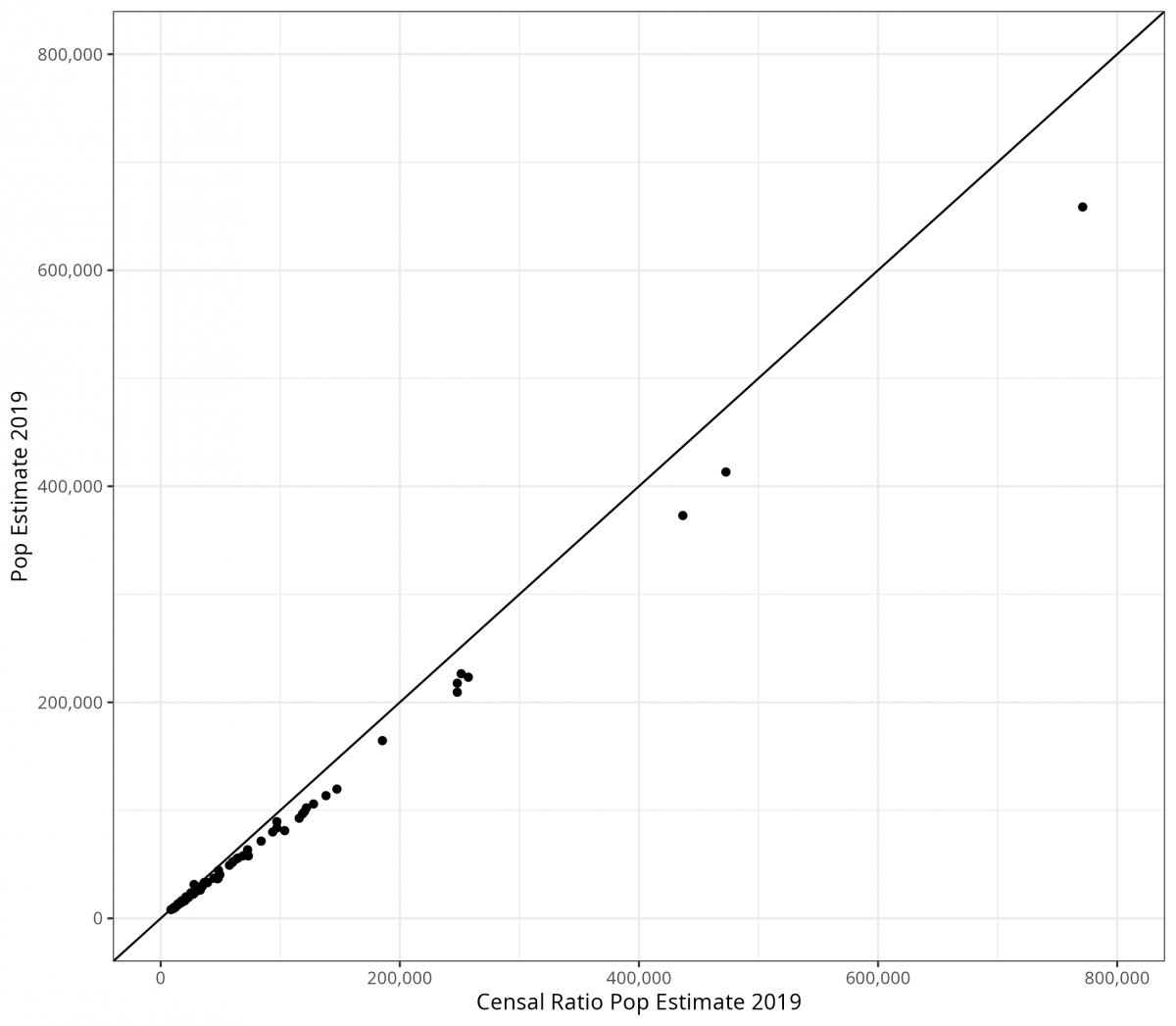
Population estimation is generally a straightforward process: any population must result from a past population number plus the births minus the deaths plus the net migration. This cohort-component method is often considered the ‘gold standard’ for population estimation (Gerland, 2014). However, the components of change (births, deaths, migrants) used to forecast a future population are… Read More
Estimating time points of significant change in cause-specific mortality: Joinpoint regression in R
![Two plots of mortality rates for six major causes of death in the United States from 1900-1998: accidents, cancer, heart disease, influenza and pneumonia, stroke, and tuberculosis. The left image is age-adjusted mortality rates for the time period, showing a notable large increase and then decrease of heart disease and other various trends for the other causes. The right image is the log transformations of these mortality rates, showing a notable dramatic decrease in tuberculosis mortality, specifically.](https://population-dynamics-lab.csde.washington.edu/wp-content/uploads/2022/10/TVD_plot1-1200x800.png)
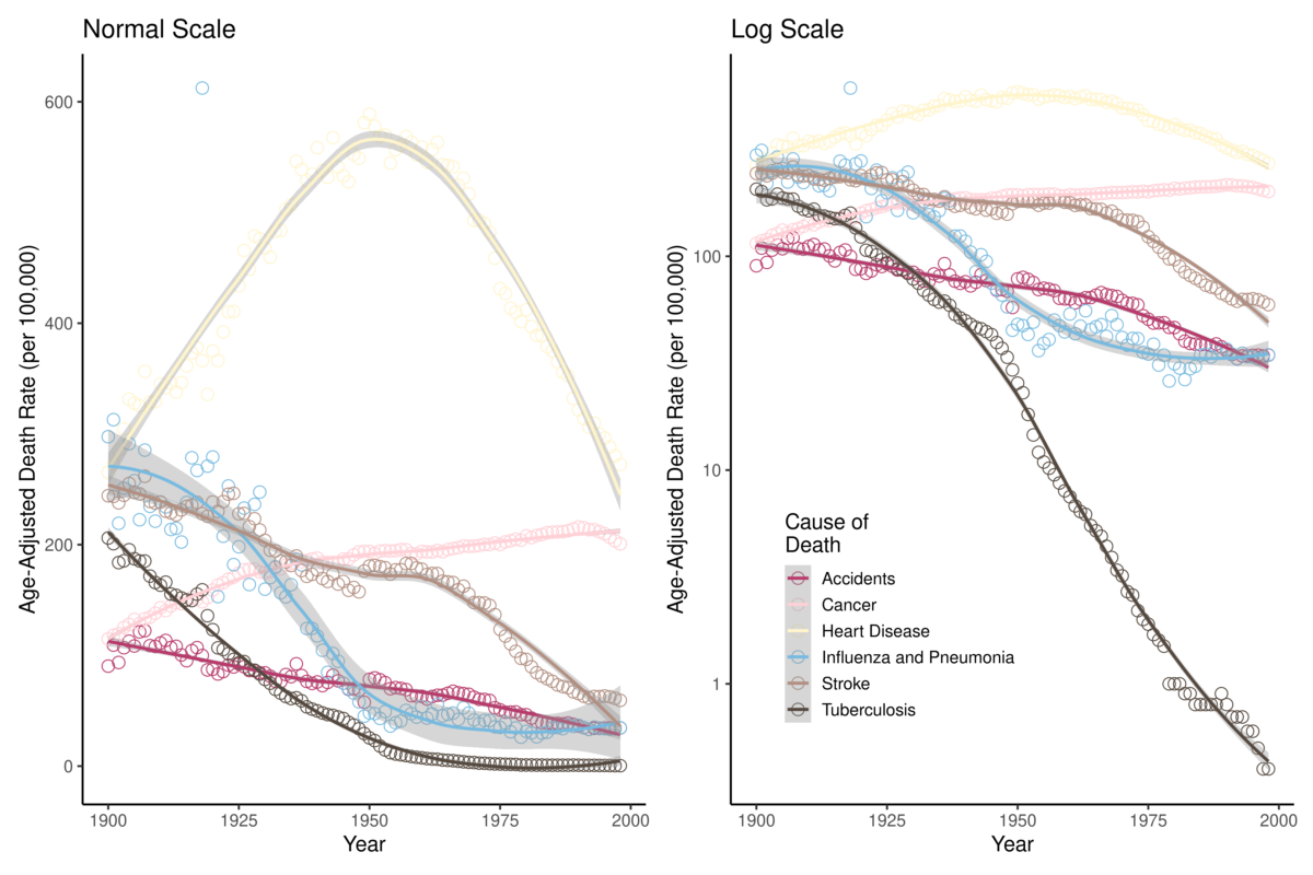
INTRODUCTION Those engaged in demographic research are often interested in how and why the vital demographic processes (fertility, mortality, and migration) change in response to certain ecological, cultural, or behavioral stimuli. Today, in the midst of a global pandemic event, epidemiologists and demographers may be interested in the ability to identify points over time during… Read More